Architecture & Customizability¶

PRGA Tile Grid¶

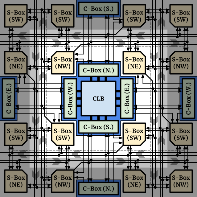
The figure above shows PRGA’s grid. Each tile in the grid (not to be confused with Tile) contains four Switch Box slots (one per corner) and one Tile slot (the blue cross-shaped box wrapping the CLB and the C-Boxes). The Tile slot contains four Connection Box slots (one per edge) and one block slot. Note that we are using the word “slot” here, because the actual usage depends on the architecture. For example, a 2x2 block occupies 4 block slots, and obstructs certain switch box and connection box slots.

TODO: explain why we need the redundant slots. In a nutshell, the redundant slots are related to design regularity and silicon implementation flexibility.

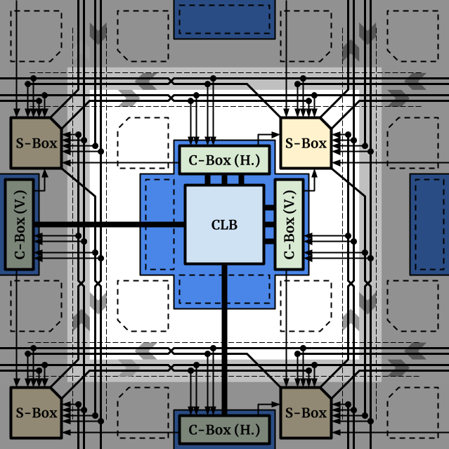
It’s still possible to emulate the conventional FPGA grid which contains only one connection box per routing channel, and one switch box per routing channel crosspoint. This is done by leaving the unused slots empty, as shown in the figure below.

Conventional FPGA Grid Emulated by the PRGA Tile Grid

Module View¶

Before diving into each type of modules listed above, let’s get familiar with an important concept in PRGA first: Module Views (ModuleView).

The ultimate goal of PRGA’s FPGA Design flow is to generate synthesizable RTL (register-transfer level) Verilog for a customized FPGA architecture, and produce FPGA CAD scripts (NOT ASIC implementation scripts) that correspond to the FPGA. However, FPGA CAD tools only need, and only take, a functional abstraction of the FPGA, ignoring most of the implementation details. For example, different modes of a multi-modal Logic Primitive are typically modeled as different blocks in VPR despite that the whole primitive is usually a single module in RTL. The figure below shows a fracturable LUT3 that can be used as two LUT2 s with shared inputs.

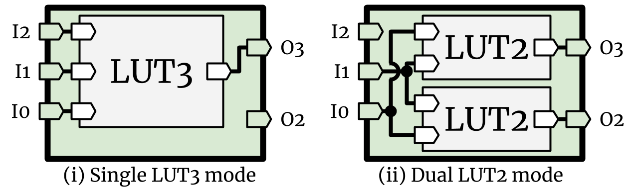
Abstract modes of Fracturable LUT3

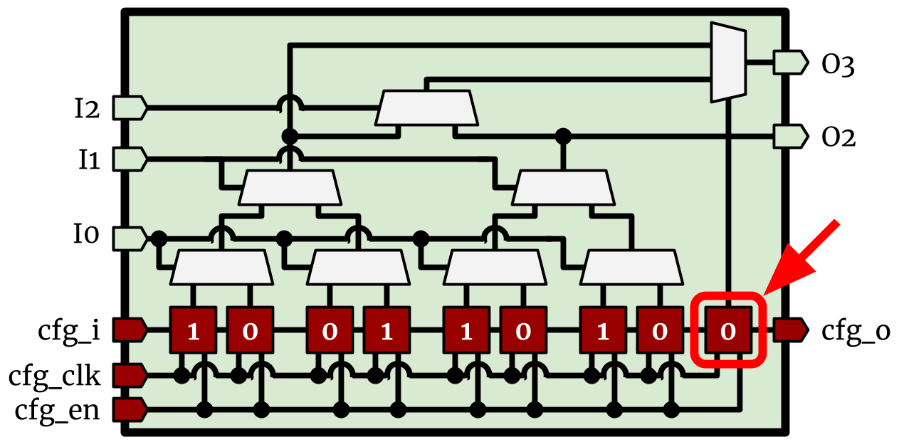
Design view (schematic) of Fracturable LUT3. Mode selection bit highlighted by red circle

To incorporate various information needed by different third-party tools, PRGA adopts the concept of View s widely used in the EDA world. Each module may have different views, and different views are used in different steps.

Currently, PRGA uses two views: ModuleView.abstract, and ModuleView.design.

Abstract View¶

The abstract view describes the nets, connections and logic of a module that are used and visible to the implemented application. It is mostly used during the Architecture Customization step, and in FPGA CAD script generation passes.

Modules in the abstract view have the following features:

Allows any net to be driven by multiple drivers. PRGA uses this to represent reconfigurable connections.
Does not contain configuration nets or modules.

Design View¶

The design view is used in RTL generation, therefore contains accurate information about all the nets and modules in the FPGA. Except for Logic Primitive s, the design view of most modules is generated by the Translation pass based on the user-specified abstract view, and then completed by the *.InsertProgCircuitry pass.

Access Modules in Different Views¶

To access modules in different views, simply add the ModuleView when you access the database property of a Context object.

abstract_lut4 = ctx.database[ModuleView.abstract, "lut4"]
design_lut4 = ctx.database[ModuleView.design, "lut4"]

Logic Primitive¶

Logic Primitive, also known as logic elements or logic resources, are the building blocks of FPGAs. In PRGA, all hard logic that can be targeted by technology mapping and synthesis are categorized as Logic Primitive s, including but not limited to LUTs, flip-flops, hard arithmetic units, SRAM macros, or even complex IP cores like memory controllers, hard processors, etc. They also correspond to the leaf-level pb_type s in VPR’s terminology.

Logic Primitive Types¶

Logic primitives are further classified into three types:

Non-Programmable primitives. They are hard components that are used in the application as is, e.g. simple flip-flops. Their abstract view and design view are typically very similar or even the same.
Programmable primitives. Their functionality is programmable. Currently only LUTs belong to this category.
Multi-Modal primitives. They have multiple modes, each emulating one or multiple other primitives. One and only one of the modes can be activated and used after the FPGA is programmed. Multi-Modal primitives are not directly targeted by synthesis. Instead, logic primitives emulated by their modes are targeted by synthesis, and eventually mapped back to the multi-modal primitives during the packing step of the RTL-to-bitstream flow. They are usually one single module in the design view, but may contain multiple submodules in the abstract view, making the two views very different.

These types are only conceptual categories and not explicitly implemented in the PRGA API.

Module Views of Logic Primitives¶

As explained in the Module View section, each logic primitive has two views: the abstract view and the design view. Most logic primitives are associated with two RTL Verilog files, each corresponding to one of the two views. The RTL corresponding to the abstract view is used during synthesis and post-synthesis simulation. The RTL corresponding to the design view is the one used in the final ASIC-compatible RTL, i.e. the one that will eventually be mapped onto transistors on your chip.

A good example is the lut.lib.tmpl.v and lut.tmpl.v pair for LUTs. Both the files might seem a bit strange, because they are file rendering templates (reference: File Rendering), not the final RTL.

lut.lib.tmpl.v

(abstract view)

// Automatically generated by PRGA's RTL generator
`timescale 1ns/1ps
module {{ module.vpr_model }} #(
    parameter   WIDTH   = 6
    , parameter LUT     = 64'b0
) (
    input wire [WIDTH - 1:0] in
    , output reg [0:0] out
    );

    always @* begin
        out = LUT >> in;
    end

endmodule

lut.tmpl.v

(design view)

// Automatically generated by PRGA's RTL generator
{% set width = module.ports.in|length -%}
`timescale 1ns/1ps
module {{ module.name }} (
    input wire [{{ width - 1 }}:0] in
    , output reg [0:0] out

    , input wire [0:0] prog_done
    , input wire [{{ 2 ** width }}:0] prog_data
        // prog_data[ 0 +: {{ 2 ** width - 1}}]: LUT content
        // prog_data[{{ 2 ** width }}]: LUT enabled (not disabled)
    );

    localparam  IDX_LUT_ENABLE = {{ 2 ** width }};

    always @* begin
        if (~prog_done || ~prog_data[IDX_LUT_ENABLE]) begin
            out = 1'b0;
        end else begin
            case (in)
                {%- for i in range(2 ** width) %}
                {{ width }}'d{{ i }}: out = prog_data[{{ i }}];
                {%- endfor %}
            endcase
        end
    end

endmodule

Some multi-modal primitives may not have the RTL for the abstract view, because their abstract view is composed of other primitives. Moreover, there are abstract -only primitives as well, often used as part of a single mode of a multi-modal primitive. FLE6 (design view RTL: fle6.tmpl.v) and its submodule, adder (abstract view RTL: adder.lib.tmpl.v are a good example.

To learn more, check out the PicoSOC tutorial.

Logic Primitives in Synthesis¶

There are three ways that logic primitives are used during technology mapping and synthesis:

Explicit Instantiation: The abstract view of a logic primitive may be directly instantiated in the application RTL. Yosys will treat explicitly instantiated logic primitives as black boxes and leave them as is in the synthesized netlist. To learn more, check out the PicoSOC tutorial.
Technology Mapping: High-level operations used in the application (for example, additions, multiplications, rising-edge-triggered non-blocking assignments) may be implemented with logic primitives via technology mapping. To enable this during synthesis, we need to provide Yosys some extra technology mapping rules (which are also written in Verilog and pretty confusing at the beginning). For example, to enable the technology mapping onto the adder primitive (abstract view RTL: adder.lib.tmpl.v), we provive Yosys with the technology mapping rule file adder.techmap.tmpl.v, which defines a set of rules to map additions, subtractions, comparisons to adder s. To learn more, check out the PicoSOC tutorial, and check out the documentation of Yosys.
Logic Synthesis: After technology mapping, the remaining logic has no choice but to be synthesized to LUTs.

Slice¶

Slices are optional levels of hierarchy between Logic Primitive s and Logic and IO Block s. They correspond to the intermediate levels of pb_type in VPR’s terminology.

As a user, you only need to describe the abstract view of a slice. The design view will be automatically generated by the Translation pass, and configuration memory will be automatically inserted by the *.InsertProgCircuitry passes. RTL will only be generated for the design view.

Logic and IO Block¶

Logic blocks and IO blocks are clusters of Slice s and Logic Primitive s with programmable local interconnects. They correspond to the top-level pb_type s in VPR’s terminology.

Logic and IO Blocks in Packing¶

As explained in the Logic Primitive section, an application RTL is first synthesized to a netlist composed of Logic Primitive s and wire connections. Then, during the packing step, the Logic Primitive s are clustered and packed into blocks, which will be placed and routed onto the physical fabric later in the RTL-to-bitstream flow. The quality of the packing result determines the utilization rate of the logic resources that are physically on your chip, and determines the difficulty of the placement and routing steps.

Connection and Switch Box¶

Work in progress.

Tile¶

Work in progress.

Array¶

Work in progress.